5 Simulation

Author

X Y (Chair)

5.1 Summary

In this book Regression and Other Stories and in practice Gelman et all. use simulation for different reasons:
- use probability models to mimic variation in the world (tools of simulation can help us better to understand how this variation plays out);
- use simulation to approximate the sampling distribution of data and propagate this to the sampling distribution of statistical estimates and procedures;
- regression models are not deterministic; they produce probabilisitc predictions. Simulation is the most convenient and general way to represent uncertainties in forecasts.

Because of this, chapter 5 introduces simulations (basic ideas and tools to perform it in R).

There are many settings where it makes sense to use a set of simulation draws to summarize a distribution, which can represent a simulation from a probability model, a prediction for a future outcome from a fitted regression, or uncertainty about parameters in a fitted model.

In this book they use the Bayesian simulation approach for regression models. Bootstrap is also a simulation approach, but it is not as general as Bayesian simulation. It is very general, any estimate can be simulated, and it is easy to use with complex models. But it has limitations (for example leading to an answer with an inappropriately high level of certainty). This method is not used in the book.

5.2 Presentation

Different examples of simulations of discrete, continuous, and mixed discrete/ continuous models are presented in this chapter.

It starts with a discrete model example: Across the world the probability a baby will be born a girl is about \(48.8\%\), with the probability of a boy then being about \(51.2\%\). If you wanted to get a sense of how many girls you’d expect out of 400 births, you could simulate using the rbinom() function.

set.seed(5)
# use set seed here because we want to get the same results every time we run the code

rbinom(n = 1, size = 400, prob = 0.488)

[1] 188

Graph results of 10000 simulations:

library(tidyverse)

── Attaching core tidyverse packages ──────────────────────── tidyverse 2.0.0 ──
✔ dplyr     1.1.4     ✔ readr     2.1.5
✔ forcats   1.0.0     ✔ stringr   1.5.1
✔ ggplot2   3.4.4     ✔ tibble    3.2.1
✔ lubridate 1.9.3     ✔ tidyr     1.3.0
✔ purrr     1.0.2     
── Conflicts ────────────────────────────────────────── tidyverse_conflicts() ──
✖ dplyr::filter() masks stats::filter()
✖ dplyr::lag()    masks stats::lag()
ℹ Use the conflicted package (<http://conflicted.r-lib.org/>) to force all conflicts to become errors

set.seed(5)
# set the global plotting theme
theme_set(theme_linedraw() +
            theme(panel.grid = element_blank()))

# set the seed
set.seed(5)

# simulate
tibble(girls = rbinom(n = 10000, size = 400, prob = .488)) %>% 
  
# plot
ggplot(aes(x = girls)) +
geom_histogram(binwidth = 2) +
scale_x_continuous("Number of girls out of 400 single births \ 
                   in 10.000 observations", breaks = 7:9 * 25) +
scale_y_continuous(expand = expansion(mult = c(0, 0.05)))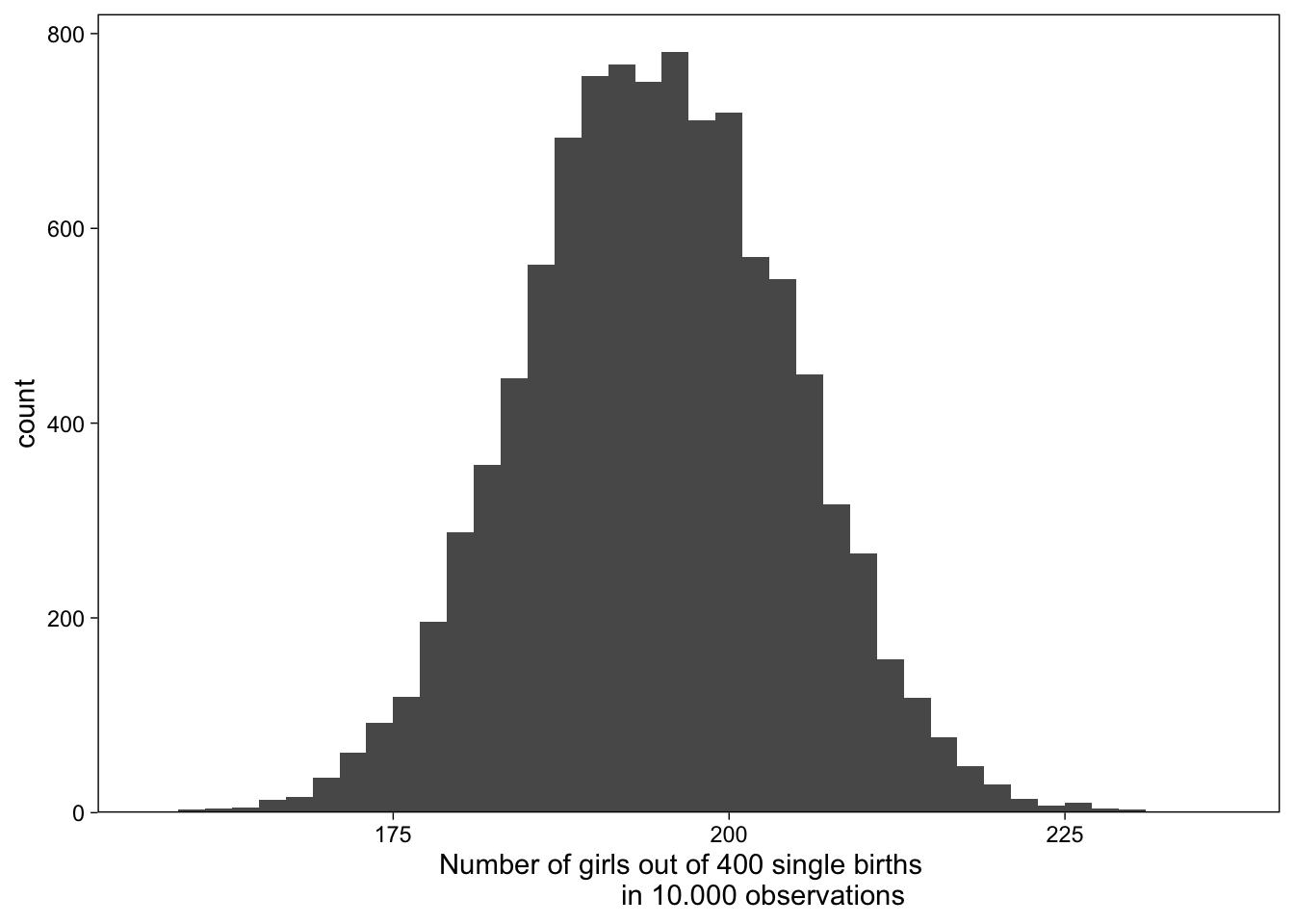

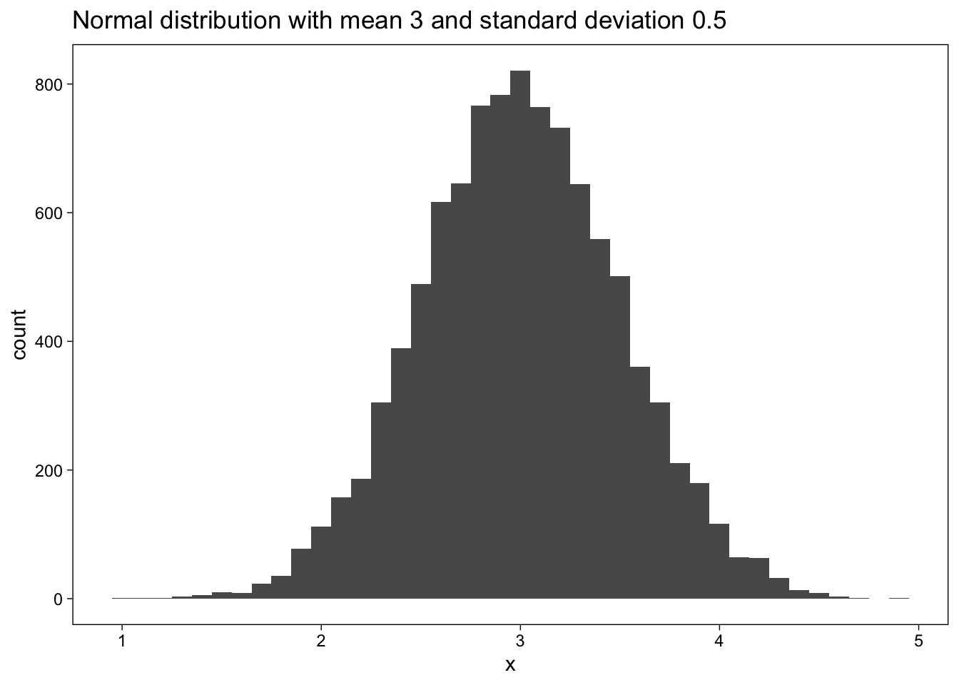
Also simulations of other models are presented. For example, the normal, binomial and Poisson distributions are presented.

Define mean=3 and sd=0,5

mean = 3
sd = 0.5
n_sims = 10000

Plot the results of 10000 simulations of a normal distribution with mean=3 and sd=0,5:

Then plot the results in histograms:

library(tidyverse)

set.seed(660)

d <- tibble(x = rnorm(n_sims, mean = mean, sd = sd))

d %>% 
  ggplot(aes(x)) +
  geom_histogram(binwidth = 0.1) +
  labs(
    title =
      str_glue(
        "Normal distribution with mean {mean} and standard deviation {sd}"
      )
  )

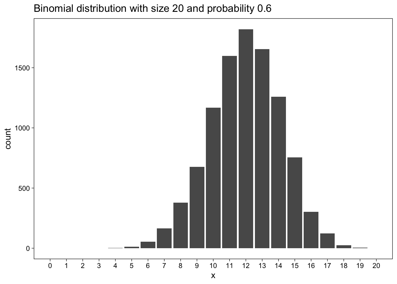
Here data for a binomial distribution:

size <- 20
prob <- 0.6

Let us plot the results of 10000 simulations of a binomial distribution with size=20 and prob=0.6:

set.seed(660)

d <- tibble(x = rbinom(n_sims, size = size, prob = prob))

d %>% ggplot(aes(x)) +
  geom_bar() +
  scale_x_continuous(breaks = seq(0, size), minor_breaks = NULL) +
  coord_cartesian(xlim = c(0, size)) +
  labs(
    title =
      str_glue(
        "Binomial distribution with size {size} and probability {prob}"
      )
  )

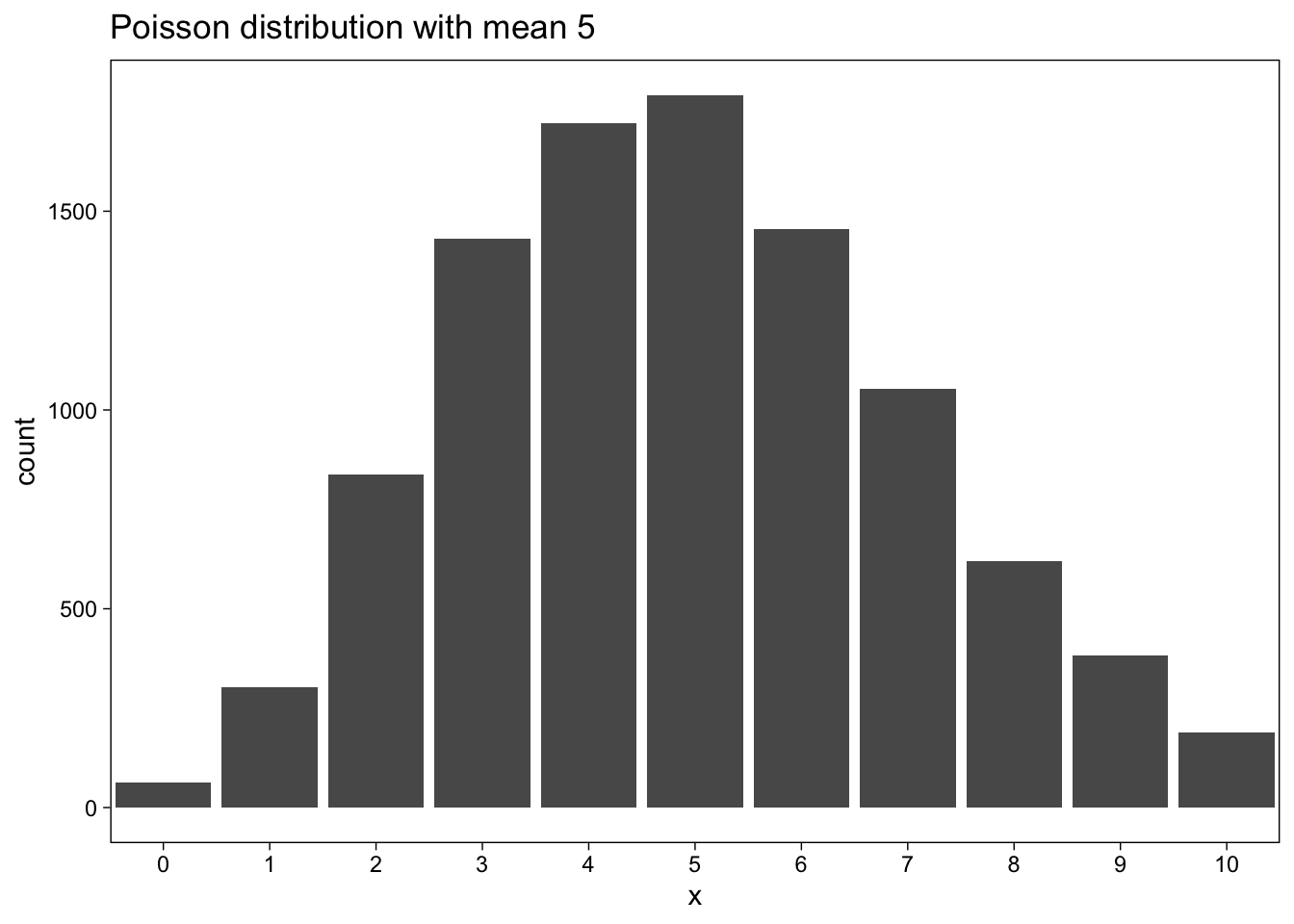
Now a Poisson distribution with mean 5:

lambda <- 5

set.seed(660)

d <- tibble(x = rpois(n_sims, lambda))

d %>% ggplot(aes(x)) +
  geom_bar() +
  scale_x_continuous(breaks = seq(0, 2 * lambda), minor_breaks = NULL) +
  coord_cartesian(xlim = c(0, 2 * lambda)) +
  labs(
    title = str_glue("Poisson distribution with mean {lambda}")
  )

Here you find a tidyverse oriented flow, as Kurz defined it.

set.seed(5)

tibble(z = rnorm(1e4, mean = 5, sd = 2)) %>% 
  summarise(mean   = mean(z),
            median = median(z),
            sd     = sd(z),
            mad_sd = mad(z))

# A tibble: 1 × 4
   mean median    sd mad_sd
  <dbl>  <dbl> <dbl>  <dbl>
1  5.00   4.99  2.02   2.03